What Is Linear Regression?

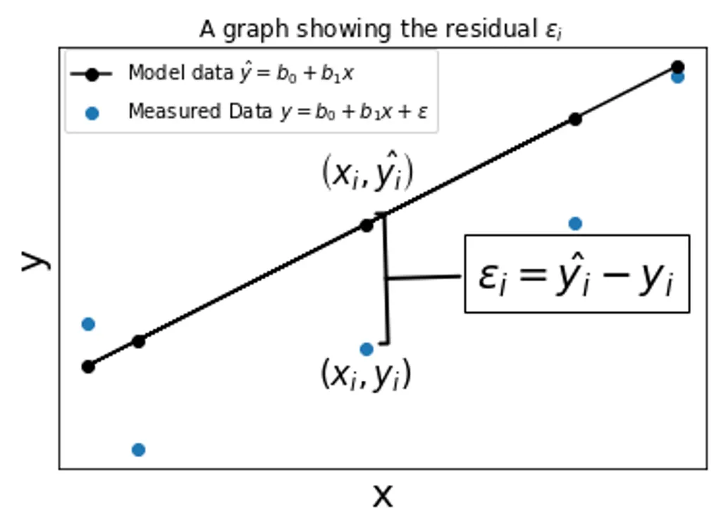
Imagine we had some data points like the plot below. The blue represents the data we measured and recorded, and the black line indicates a hypothetical line that best represents the data.

Why do we want to find this line? Well, if we knew the equation for a line that ran right in the middle of our data, predict any value using the equation of such a line with reasonable accuracy.

from sklearn.datasets import make_regression
import matplotlib.pyplot as plt
from sklearn import linear_model
from sklearn.model_selection import train_test_split

# Generate regression dataset
X, y = make_regression(n_samples=1000, n_features=1, noise=35, random_state=1)
# split data/targets into test/train
X_train, X_test, y_train, y_test = train_test_split(X, y, test_size=0.33, random_state=42)

# Create linear regression object
regr = linear_model.LinearRegression()

# Train the model using the training sets
regr.fit(X_train, y_train)

# Make predictions using the testing set
y_pred = regr.predict(X_test)

fig, ax = plt.subplots()
ax.scatter(X_test, y_test)
ax.plot(X_test, y_pred, color='black')
ax.legend(['predicted value','measured data'])
# for major ticks
ax.set_xticks([])
# for minor ticks
ax.set_xticks([], minor=True)
# for major ticks
ax.set_yticks([])
# for minor ticks
ax.set_yticks([], minor=True)
ax.set_xlabel('x', fontsize=20)
ax.set_ylabel('y', fontsize=20)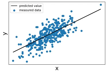

A simple Linear Regression model takes the form below

$y = b_0 + b_1x + \epsilon$

where:

• $y$ is our response variable, i.e. the dependant variable, the value we are trying to predict
• $x$ is the regressor variable, i.e. the independant variable. It is assumed to be measured with neglible error.
• $\epsilon$ is a random error term that we cannot directly measure, however we assume it exists an accounts for any inacuraccies in our model
• $b_0$​ is the bias, i.e. the y intercept of the linear regression line
• $b_1$​ is the slope of the regression line

$b_0$​ and $b_1$​ are the values we are trying to find in a Simple Regression model, and they are assumed to be constant values and not functions of $x$, which makes the equation linear.

The random error term $\epsilon$ has expected value (mean) of zero, and constant variance.

• $E(\epsilon) = 0$
• $Var(\epsilon) = \sigma^2$

How does it work? Based on our assumed model, there is some error corresponding to each data point. This extra error is called the residual.

# Generate regression dataset
X, y = make_regression(n_samples=15, n_features=1, noise=20, random_state=5)
# split data/targets into test/train
X_train, X_test, y_train, y_test = train_test_split(X, y, test_size=0.33, random_state=42)

# Create linear regression object
regr = linear_model.LinearRegression()

# Train the model using the training sets
regr.fit(X_train, y_train)

# Make predictions using the testing set
y_pred = regr.predict(X_test)


fig, ax = plt.subplots()
ax.set_title('A graph showing the residual $\epsilon_i$')
ax.scatter(X_test, y_test)
ax.plot(X_test, y_pred, color='black', marker='o')
ax.legend([r'Model data $\hat{y}=b_0 + b_1 x$', r'Measured Data $y=b_0 + b_1 x + \epsilon$'], bbox_to_anchor=(0.6,1.02))
fs = 14
ax.annotate('$\epsilon_i = \hat{y_i} - y_i$', xy=(0.5, 0.45), xytext=(0.8, 0.4), xycoords='axes fraction',
            fontsize=fs*1.5, ha='center', va='bottom', rotation=0,
            bbox=dict(boxstyle='square', fc='white'),
            arrowprops=dict(arrowstyle='-[, widthB=1.6, lengthB=0.2', lw=2.0))

ax.annotate(r'$\left( x_i, \hat{y_i} \right)$', xy=(0.4, 0.68), xycoords='axes fraction', fontsize=fs*1.2)
ax.annotate(r'$\left( x_i, y_i \right)$', xy=(0.4, 0.2), xycoords='axes fraction', fontsize=fs*1.2)
# for major ticks
ax.set_xticks([])
# for minor ticks
ax.set_xticks([], minor=True)
# for major ticks
ax.set_yticks([])
# for minor ticks
ax.set_yticks([], minor=True)
ax.set_xlabel('x', fontsize=20)
ax.set_ylabel('y', fontsize=20)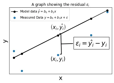

We wish to make the sum total of the error for all of the data points as small as possible. In other words, we are minimizing the residual.

One method is to square the sum of the residuals, since having a negative value is undesirable as it instead subtracts from the total amount of error, which can be misleading. We can right the Sum of Squared Errors (SSE) like so.

If we have $n$ data points, the total squared error is

$SSE(b_0,b_1) = \sum\limits_{i}^{n} \epsilon_i^2 = \sum\limits_{i}^{n}\left(\hat{y}_i - y_i\right)^2 = \sum\limits_{i}^{n}\left(b_0 + b_1x - y_i\right)^2$

Minimizing this function with respect to b0b0​ and b1b1​ is the same as taking the partial derivatives with respect to each and setting them each to zero. This results in two equations with two unkowns (once you sum over all the x and y values). The two equations is referred to as the Normal Equations.

$\frac{\partial{SSE}}{\partial{b_0}} = 2\sum\limits_{i}^{n}\left(b_0 + b_1x - y_i\right) = 0$

$\frac{\partial{SSE}}{\partial{b_1}} = 2\sum\limits_{i}^{n}\left(b_0 + b_1x - y_i\right)x = 0$

These equations can be expressed as:

$nb_0 + b_1 \sum\limits_{i}^{n} x_i = \sum\limits_{i}^{n} y_i$

$b_0 \sum\limits_{i}^{n} x_i + b_1 \sum\limits_{i}^{n} x_i^2 = \sum\limits_{i}^{n} x_iy_i$

$$\begin{bmatrix} n & s_x \\ s_x & s_{xx} \end{bmatrix} \begin{bmatrix} b_0 \\ b_1 \end{bmatrix} = \begin{bmatrix} s_y \\ s_{xy} \end{bmatrix}$$ $$A b = v$$

Example:

import numpy as np

# Generate regression dataset
x, y = make_regression(n_samples=1000, n_features=1, noise=35, random_state=1)
# Create linear regression object
regr = linear_model.LinearRegression()
# Train the model using the training sets
regr.fit(x,y)

x = x.reshape((1000,))

n = len(x)
s_x = sum(x)
s_xx = sum(x*x)
s_y = sum(y)
s_xy = sum(x*y)

print('n = {}'.format(n))
print('s_x = {0:.{1}f}'.format(s_x, 4))
print('s_y = {0:.{1}f}'.format(s_y, 4))
print('s_xx = {0:.{1}f}'.format(s_xx, 4))
print('s_xy = {0:.{1}f}'.format(s_xy, 4))

• n = 1000
• s_x = 38.8125
• s_y = 2488.7840
• s_xx = 963.8755
• s_xy = 36596.1745

The equations reduce down to:

$1000b_0 + 38.8125 b_1 = 2488.7840$

$38.8125 b_0 ​+ 963.8755 b_1​=36596.1745$

Even though it is a linear system with only two equations. Numpy can solve it for us.

A = np.array([[n, s_x],[-s_x, s_xx]])
b = np.array([s_y, s_xy])

v = np.linalg.solve(A,b)

# We get approximately the same results
print("solution by solving linear system")
print("b_0 = {}".format(v[0]))
print("b_1 = {}".format(v[1]))

print()
print("solution using scikit-learn")
print("b_0 = {}".format(regr.intercept_))
print("b_1= {}".format(regr.coef_))

solution by solving linear system

• b_0 = 1.0135779148091075
• b_1 = 38.00855317991723

solution using scikit-learn

• b_0 = 1.0167510469725556
• b_1 = 37.92679771

We get aproximately the same solutions.

Conclusion

We are not quite done yet. Because $\epsilon_i$ is a random stochastic term meant to represent error in our measurements, it will not be the same each time we collect our data. This means the $\hat{y}_i$​, our predicted value, will change each time as well. This in turn means our $b_0$​, $b_1$ values will be different each time as well.

In other words, each time we collect our data, due to random errors in the measurements, we would need a completely different regression line to represent the new values.

How to get around this? Well what we can do is essentially find the average values of $b_0$​ and $b_1$​ as we take more and more measurements. This will give us a more accurate fit.